import sympy as sy
from scipy.optimize import fsolve
import sympy as sy

import pandas as pd
import numpy as np
import matplotlib.pyplot as plt
from pandas_datareader import data
import datetime as dt

from statsmodels.graphics.tsaplots import plot_acf
from statsmodels.graphics.tsaplots import acf as acf_func
from statsmodels.graphics.tsaplots import plot_pacf
from statsmodels.tsa.arima_process import ArmaProcess
from statsmodels.tsa.arima.model import ARIMA


plt.style.use("ggplot")

import warnings

warnings.filterwarnings("ignore")
Lag operator is a type of linear operator especially convenient in time series analysis, it has all properties that a linear operator should have.
Consider an infinite time series \(\{y_t\}^{\infty}_{t=-\infty}\), we operate with one lag is denoted as
\[ Ly_t = y_{t-1} \]
Lag twice or three times
\[ L^2y_t = y_{t-2},\qquad L^3y_t = y_{t-3} \]
Or a polynomial lag operation
\[ (1- 3L)(2+4L)(1+2L)y_t \]
It would be easier to demonstrate with SymPy’s algebraic capacity:
L = sy.symbols("L")
poly = (1 - 3 * L) * (2 + 4 * L) * (1 + 2 * L)
poly.expand()
\(\displaystyle - 24 L^{3} - 16 L^{2} + 2 L + 2\)
Operate on \(y_t\)
\[ (- 24 L^{3} - 16 L^{2} + 2 L + 2)y_t = -24y_{t-3}-16y_{t-2}+2y_{t-1}+2y_t \]
\(1st\)-Order Difference Equations
Start with
\[ y_t = \phi y_{t-1}+u_t \]
Use lag operator and rearrange \[ y_t-\phi L y_t = u_t\qquad\longrightarrow\qquad(1-\phi L)y_t = u_t \]
That mean it must be an inverse of \((1-\phi L)\) which achieves \[ \begin{align} (1-\phi L)^{-1}(1-\phi L)y_t&=(1-\phi L)^{-1}u_t\\ y_t&=(1-\phi L )^{-1}u_t \end{align} \]
How do we find out what \((1-\phi L)^{-1}\) is?
Fortunately, we have encountered this type of series in high school, \((1-\phi L)^{-1}\) can be expanded into an infinite geometric series
\[ \frac{1}{1-\phi L} = 1 + \phi L + \phi^2L^2 + \phi^3L^3 + \cdots =\sum_{i=0}^\infty (\phi L)^i \]
Rewrite equation \((1)\)
\[ y_t = (1 + \phi L + \phi^2L^2 + \phi ^3L^3 + \cdots)u_t = u_t +\phi u_{t-1}+\phi ^2u_{t-2} + \phi ^3u_{t-3}+\cdots \]
However, though we start from $y_t = y_{t-1}+u_t $ and derived \((2)\), they are not essential consistent.
Because recall the solution of the \(1st\) order difference equation by recursive substitution
\[ y_t = \phi ^t y_0 + \phi ^{t-1}u_{1} + \phi ^{t-2}u_{2} +\phi ^{t-3}u_{3} + ... + \phi u_{t-1} + u_t \]
Obviously, if you substract \((3)\) from \((2)\), it doesn’t get a \(0\).
The the leftover infinite series has high powers on \(t\), they converge to \(0\) on condition that \(|\phi|<1\), therefore the only missing term is \(\phi ^ty_0\).
But we can still that the equation \((1)\) holds \[\begin{align} y_t &= \phi^ty_0 + (1-\phi L)^{-1}u_t\\ (1-\phi L)y_t &= (1-\phi L)\phi^ty_0 + (1-\phi L)(1-\phi L)^{-1}u_t\\ & = \phi^ty_0 -\phi\phi^{t-1}y_0 + u_t\\ &=u_t \end{align}\] We proved $y_t=(1-L)^{-1}u_t $, here we assume that \(y_0\) is an initial condition which is a constant, which guarantees \(Ly_0 = y_0\).
\(2nd\)-Order Difference Equations
Consider a \(2nd\)-order difference equation:
\[ y_t=\phi_1y_{t-1}+\phi_2y_{t-2}+u_t \]
In lag operator form
\[ (1-\phi_1L-\phi_2L^2)y_t=u_t \]
The polynomial on the LHS can be factored
\[ 1-\phi_1L-\phi_2L^2 = (1-\lambda_1 L)(1-\lambda_2 L) = 1-(\lambda_1+\lambda_2) L + \lambda_1\lambda_2 L^2 \]
The parameters of polynomial can be pinned down by a system of nonlinear equations \[ \begin{align} \lambda_1+\lambda_2 &= \phi_1\\ \lambda_1\lambda_2&=-\phi_2 \end{align} \]
Assume the model is \[ y_t=0.9y_{t-1}+0.3y_{t-2}+u_t \]
Solve the system of nonlinear equations with fsolve
def func(lamda):
    lamda1, lamda2 = lamda[0], lamda[1]
    F = np.empty(2)
    F[0] = lamda1 + lamda2 - 0.9
    F[1] = lamda1 * lamda2 + 0.3
    return F


lamda_guess = np.array([0, 0])  # [1, 1] is initial value
lamda1, lamda2 = fsolve(func, lamda_guess)
print("lambda1 : {:.4f}, lambda2: {:.4f}".format(lamda1, lamda2))
lambda1 : 1.1589, lambda2: -0.2589\[ 1-0.9L-0.3L^2 = (1-\underbrace{1.1589}_{\lambda_1} L)(1+\underbrace{0.2589}_{-\lambda_2} L) \]
As a reference, we post another solution from \(2nd\) order difference equation, more details are in later sections
lamda1 = (0.9 + np.sqrt(0.9**2 + 4 * 0.3)) / 2
lamda2 = (0.9 - np.sqrt(0.9**2 + 4 * 0.3)) / 2
print(
    "lambda1 and lambda2 are {0:.3f} and {1:.3f} respectively.".format(lamda1, lamda2)
)
lambda1 and lambda2 are 1.159 and -0.259 respectively.The \(\lambda\)’s here are actually the eigenvalues of the linear system if we rewrite the system into a matrix form. But don’t worry about the details yet, we will demonstrate the gory details in this chapter later.
The system \((4)\) will be stable only when both eigenvalues, \(\lambda_1\) and \(\lambda_2\)’s modulus less than \(1\), geometrically they must lie inside a unit circle, if lie on the unit circle or outside, the system is explosive.
ar_params = np.array([1, -0.8, 0.35])  # alwasy specify zero lag as 1
ma_params = np.array([1])  # alwasy specify zero lag as 1
ar2 = ArmaProcess(ar_params, ma_params)  # the Class requires AR and MA's parameters
ar2_sim = ar2.generate_sample(nsample=100)
ar2_sim = pd.DataFrame(ar2_sim, columns=["AR(2)"])
ar2_acf = acf_func(ar2_sim.values, fft=False, nlags=50)  # return the numerical ACF
fig, ax = plt.subplots(figsize=(14, 5), nrows=1, ncols=2)
ar2_sim.plot(ax=ax[0])
pd.DataFrame(ar2_acf).plot.bar(ax=ax[1], label="ACF")
plt.show()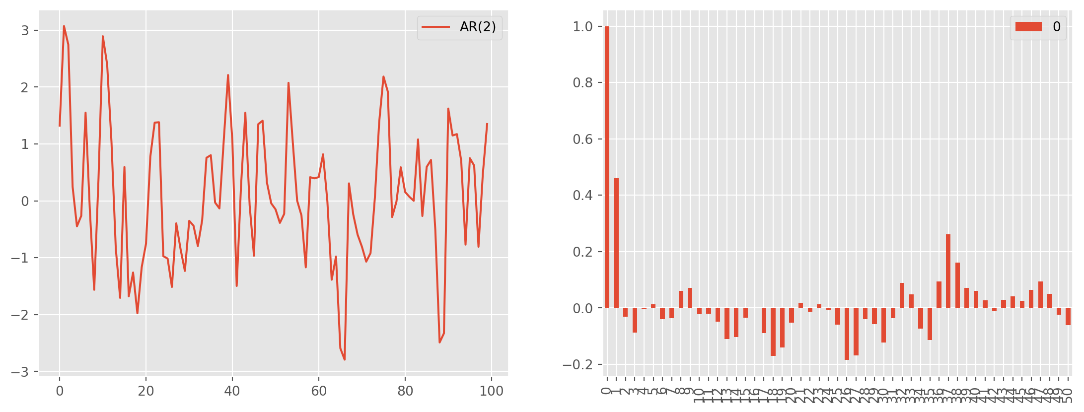
Solving \(1st\) Order Difference Equations
Now we turn to difference equations in more details, which are horses of all dynamic system researches, including time series analysis.
Difference equations are commonly solved by recursive substitution, consider the \(1st\) difference equation below, where \(u_t\) is a white noise process
\[ y_t = \phi y_{t-1} + u_t \]
and shift one period backward
\[ y_{t-1} =\phi y_{t-2} + u_{t-1} \]
Substitute back to the original equation \((1)\)
\[ y_t = \phi (\phi y_{t-2} + u_{t-1}) + u_t = \phi^2y_{t-2} + \phi u_{t-1} +u_t \]
then substitute \(y_{t-2}\),
\[ y_t = \phi^2(\phi y_{t-3} + u_{t-2}) + \phi u_{t-1}= \phi^3y_{t-3}+\phi^2u_{t-2}+\phi u_{t-1}+u_t \]
continue the recursive substitution, the solution will take form as an infinite series
\[ y_t = \phi^t y_0 + \phi^{t-1}u_{1} + \phi^{t-2}u_{2} + \phi^{t-3}u_{3} + ... + \phi u_{t-1} + u_t \]
Dynamic Multiplier
The dynamic multiplier is a partial derivative toward \(u_i,\ i \in (1,2,.., t)\), e.g. dynamic multiplier of \(u_1\)
\[ \frac{\partial y_t}{\partial u_1} = \phi^{t-1} \]
The value of \(\phi\) characterizes the pattern of the difference equation.
The charts below shows how the parameter \(\phi\) determines the system.
y = np.zeros(30)
y[0] = 100

ax_pos = [221, 222, 223, 224]
fig = plt.figure(figsize=(12, 7))
tt = ["$\phi=.9$", "$\phi=1$", "$\phi=1.3$", "$\phi=-0.8$"]
phi = [0.9, 1, 1.3, -0.8]

for j in range(4):
    ax = fig.add_subplot(ax_pos[j])
    for i in range(1, 30):
        u = np.random.randn()
        y[i] = phi[j] * y[i - 1] + u
    ax.bar(np.arange(len(y)), y)
    ax.set_title(tt[j], size=16)
plt.suptitle(r"$y_t=\phi y_{t-1}+u_t$", size=22)
plt.show()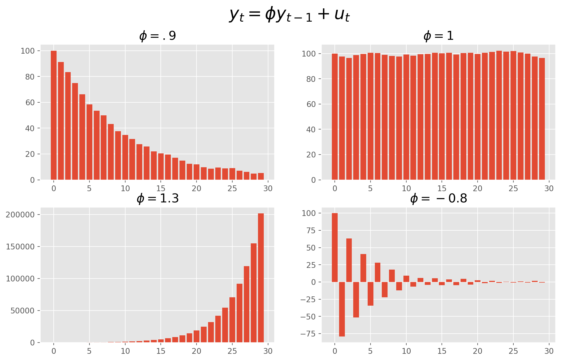
As long as \(-1<\phi<1\), the system will be stable, otherwise explosive.
Impulse Response Function of AR(1)
Impulse response function (IRF) depicts the path of \(Y\) from a unit impulse in \(u\).
For an \(\text{AR}(1)\) model, the IRF is straightforward, for example \[ Y_t = .88 Y_{t-1}+u_t \] The IRF is traced out by a recursive substitution \[ \begin{align} \text{IRF}(0)&=1\\ \text{IRF}(1)&=0.88\times \text{IRF}(0)\\ \text{IRF}(2)&=0.88\times \text{IRF}(1)\\ \text{IRF}(3)&=0.88\times \text{IRF}(2)\\ &\ldots \end{align} \] So for \(\text{AR(1)}\), the IRF is simply coefficient raise to the power of horizon \[ \text{IRF}(k)=\theta^k \]
def irf_ar1(theta, horizon, impluse=1):
    irf = [impluse]
    for i in range(0, horizon):
        irf.append(irf[-1] * theta**i)
    irf[0] = 0
    return irf
irf = irf_ar1(0.97, 20)impulse = np.zeros(len(irf))
impulse[1] = 1
fig, ax = plt.subplots(figsize=(12, 5), nrows=2, ncols=1)
ax[0].bar(np.arange(len(irf)), irf)
ax[0].bar(np.arange(len(impulse)), impulse, color="Coral")
ax[1].bar(np.arange(len(impulse)), impulse, label="Unit Impulse", color="Coral")
plt.legend()
plt.suptitle("Impluse Reponse Function of AR(1)")
plt.show()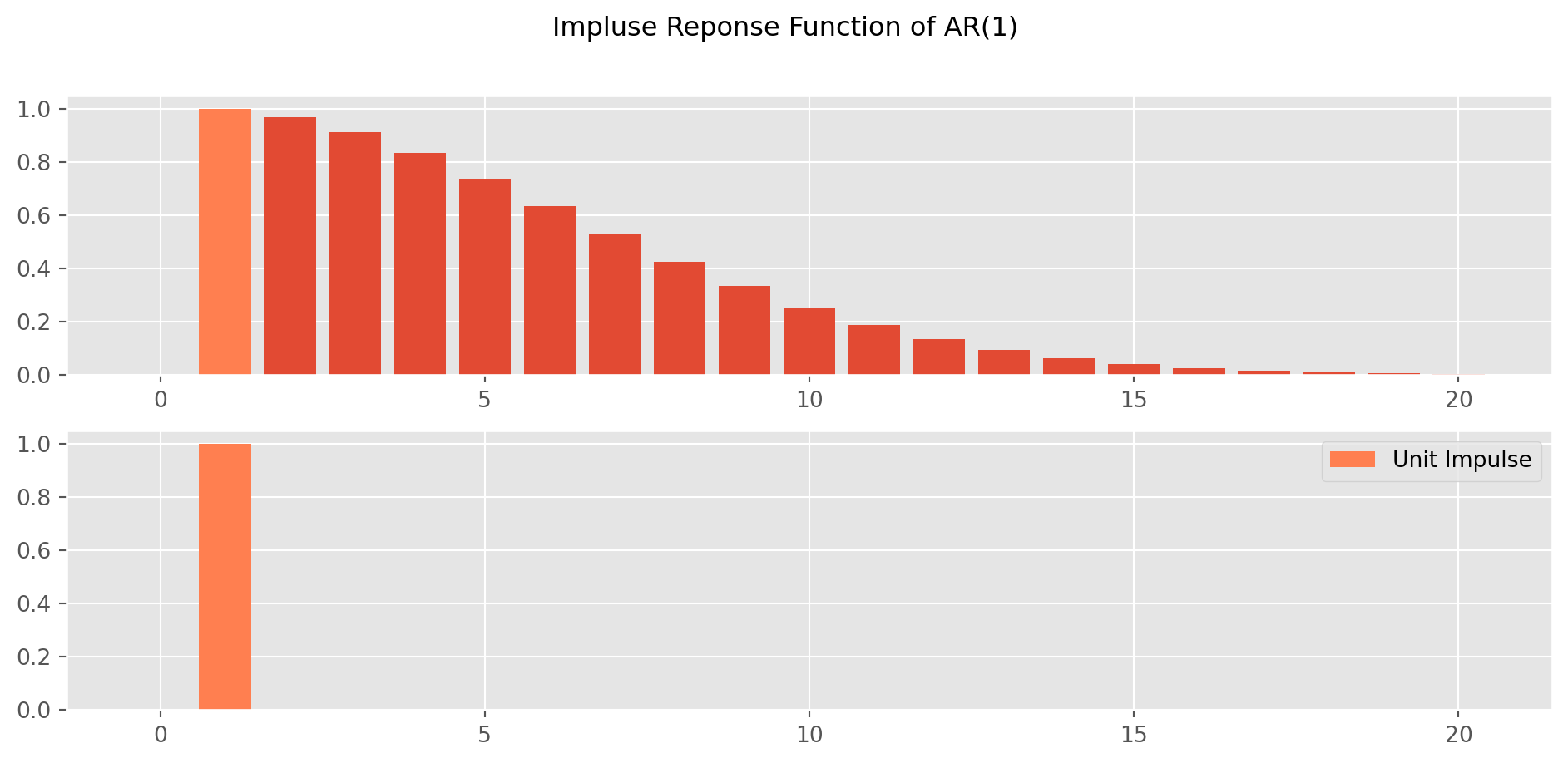
However for \(\text{AR(p)}\), the IRF is taking a confusing expression. For instance, an \(\text{AR}(3)\) model \[ Y_t = 0.94 Y_{t-1} - 0.35 Y_{t-2} -0.3 Y_{t-3} +u_t \]
\[\begin{align} \text{IRF}(0)=1&\\ \text{IRF}(1)=0.94\times \text{IRF}(0)=0.94&\\ \text{IRF}(2)=0.94 \times \text{IRF}(1)-0.35 \times \text{IRF}(0)=0.5336&\\ \text{IRF}(3)=0.94 \times \text{IRF}(2)-0.35\times \text{IRF}(1)-0.3 \times \text{IRF}(0)=-0.1274&\\ \text{IRF}(4)=0.94 \times \text{IRF}(3)-0.35 \times \text{IRF}(2)-0.3 \times \text{IRF}(1)=-0.5885\\ \text{IRF}(j)=0.94 \times \text{IRF}(j-1)-0.35\times \text{IRF}(j-2)-0.3 \times \text{IRF}(j-3)& \end{align}\]
Though this is the fundamental algorithm of IRF, rarely programs are written exactly as this recursive form.
Once we discussed the \(k\)-th order difference equation, we will see there is a way simpler approach in matrix form.
Solving \(k\)-th Order Difference Equations
Define the \(k\)-vector \(\pmb{y}_t\) by
\[ \pmb{y}_t= \left[ \begin{matrix} y_t\\ y_{t-1}\\ y_{t-2}\\ \vdots\\ y_{t-k+1} \end{matrix} \right] \]
Define the \(k\times k\) matrix \(\pmb{F}\) by
\[ \pmb{F}= \left[ \begin{matrix} \phi_1 & \phi_2 & \phi_3 &\cdots &\phi_{k-1} & \phi_k\\ 1 & 0 & 0 &\cdots &0 & 0\\ 0 & 1 & 0 &\cdots &0 & 0\\ \vdots &\vdots & \vdots& \ddots &\vdots & \vdots\\ 0 & 0 & 0 &\cdots & 1 & 0 \end{matrix} \right] \]
Last, define \(k\)-vector \(\pmb{u}_t\) by
\[ \pmb{u_t}= \left[ \begin{matrix} u_t\\ 0\\ 0\\ \vdots\\ 0 \end{matrix} \right] \]
Thus linear system in matrix form is
\[ \pmb{y}_t = \pmb{F}\pmb{y}_{t-1}+\pmb{u}_t \]
or explicitly
\[ \left[ \begin{matrix} y_t\\ y_{t-1}\\ y_{t-2}\\ \vdots\\ y_{t-k+1} \end{matrix} \right]= \left[ \begin{matrix} \phi_1 & \phi_2 & \phi_3 &\cdots &\phi_{k-1} &\phi_k\\ 1 & 0 & 0 &\cdots &0 & 0\\ 0 & 1 & 0 &\cdots &0 & 0\\ \vdots &\vdots & \vdots& \ddots &\vdots & \vdots\\ 0 & 0 & 0 &\cdots & 1 & 0 \end{matrix} \right] \left[ \begin{matrix} y_{t-1}\\ y_{t-2}\\ y_{t-3}\\ \vdots\\ y_{t-k} \end{matrix} \right] + \left[ \begin{matrix} u_t\\ 0\\ 0\\ \vdots\\ 0 \end{matrix} \right] \]
The recursive substitutions of matrix form give us a general expression
\[ \pmb{y}_t = \pmb{F}^t \pmb{y}_0 + \pmb{F}^{t-1}\pmb{u}_{1} + \pmb{F}^{t-2}\pmb{u}_{2} + \pmb{F}^{t-3}\pmb{u}_{3} + ... + \pmb{F}\pmb{u}_{t-1} + \pmb{u}_t \]
\[ \begin{aligned} \left[\begin{array}{c} y_{t} \\ y_{t-1} \\ y_{t-2} \\ \vdots \\ y_{t-k+1} \end{array}\right]=\pmb{F}^{t}\left[\begin{array}{c} y_{0} \\ y_{-1} \\ y_{-2} \\ \vdots \\ y_{-k+1} \end{array}\right]+\pmb{F}^{t-1}\left[\begin{array}{c} u_{1} \\ 0 \\ 0 \\ \vdots \\ 0 \end{array}\right]+\pmb{F}^{t-2}\left[\begin{array}{c} u_{2} \\ 0 \\ 0 \\ \vdots \\ 0 \end{array}\right] +\pmb{F}^{t-3}\left[\begin{array}{c} u_{3} \\ 0 \\ 0 \\ \vdots \\ 0 \end{array}\right]+\cdots+\pmb{F}\left[\begin{array}{c} u_{t-1} \\ 0 \\ 0 \\ \vdots \\ 0 \end{array}\right] \end{aligned} + \left[\begin{array}{c} u_{t} \\ 0 \\ 0 \\ \vdots \\ 0 \end{array}\right] \]
Dynamic Multiplier
If \(\pmb{F}\) has \(k\) distinct eigenvalues, it is possible to be diagonalized, such that
\[ \pmb{F} = \pmb{P\Lambda P}^{-1} \]
where \(\pmb{P}\) holds all the distinct eigenvectors, whereas all the distinct eigenvalues stay on the principal diagonal of \(\pmb{\lambda}\).
The eigenvalue can characterize the dynamic multiplier as we have seen for the \(1st\)-order difference equation. For instance, \(\pmb{F}^3\) is decomposed as
\[ \pmb{F}^3 = \pmb{P\Lambda P}^{-1} \pmb{P\Lambda P}^{-1} \pmb{P\Lambda P}^{-1} = \pmb{P\Lambda } \pmb{\Lambda } \pmb{\Lambda P}^{-1} =\pmb{P} \pmb{\Lambda }^3 \pmb{P}^{-1} \]
where
\[ \pmb{\Lambda }^3 = \left[\begin{array}{ccccc} \lambda_{1}^{3} & 0 & 0 & \cdots & 0 \\ 0 & \lambda_{2}^{3} & 0 & \cdots & 0 \\ \vdots & \vdots & \vdots & \ddots & \vdots \\ 0 & 0 & 0 & \cdots & \lambda_{k}^{3} \end{array}\right] \]
Therefore in general, \[ \pmb{F}^t =\pmb{P} \pmb{\Lambda }^t \pmb{P}^{-1} \]
Denote the \((i, j)\) element of \(\pmb{F}^t\) as \(f^{(t)}_{ij}\), for instance the \((4, 5)\) element of \(\pmb{F}^{t-1}\) is \(f^{(t-1)}_{45}\). The first row of system \((6)\) is
\[ y_t = f^{(t)}_{11}y_0+ f^{(t)}_{12}y_{-1} + f^{(t)}_{13}y_{-2} + \cdots + f^{(t)}_{1k}y_{-k-1} + f^{(t-1)}_{11}u_1 +f^{(t-2)}_{11}u_2 +...+f^{1}_{11}u_{t-1}+u_{t} \]
To generalize the time span
\[ y_{t+i} = f^{(i)}_{11}y_t+ f^{(i)}_{12}y_{t-1} + f^{(i)}_{13}y_{t-2} + \cdots + f^{(i)}_{1k}y_{t-k-1} + f^{(i-1)}_{11}u_t +f^{(i-2)}_{11}u_{t+2} +...+f^{1}_{11}u_{t+i-1}+u_{t+i} \]
The dynamic multiplier is
\[ \frac{\partial y_{t+i}}{\partial u_t} = f^{(i-1)}_{11} \]
We can show that dynamic multiplier is a linear combination of the power of eigenvalues.
\[ \frac{\partial y_{t+i}}{\partial u_t} = f^{(i-1)}_{11} = c_1 \lambda_1^{i-1}+c_2 \lambda_2^{i-1}+ \cdots + c_p \lambda_p^{i-1} \]
Linear Combination of Eigenvalues of \(\pmb{F}\)
If we denote \(t_{ij}\) and \(t^{ij}\) the \((i, j)\) element of \(\pmb{P}\) and \(\pmb{P}^{-1}\) respectively. \(\pmb{F}^{i-1}\) can be explicitly written as
\[ \pmb{F}^{i-1}=\left[\begin{array}{cccc} t_{11} & t_{12} & \cdots & t_{1 k} \\ t_{21} & t_{22} & \cdots & t_{2 k} \\ \vdots & \vdots & \ddots & \vdots \\ t_{k 1} & t_{k 2} & \cdots & t_{kk} \end{array}\right]\left[\begin{array}{ccccc} \lambda_{1}^{i-1} & 0 & 0 & \cdots & 0 \\ 0 & \lambda_{2}^{i-1} & 0 & \cdots & 0 \\ \vdots & \vdots & \vdots & \ddots & \vdots \\ 0 & 0 & 0 & \cdots & \lambda_{k}^{i-1} \end{array}\right]\left[\begin{array}{ccccc} t^{11} & t^{12} & \cdots & t^{1 k} \\ t^{21} & t^{22} & \cdots & t^{2 k} \\ \vdots & \vdots & \ddots & \vdots \\ t^{k 1} & t^{k 2} & \cdots & t^{k k} \end{array}\right] \]
The \((1, 1)\) element of \(\pmb{F}^{i-1}\) is
\[\begin{align} f^{(i-1)}_{11}&=\left(t_{11} t^{11}\right) \lambda_{1}^{i-1}+\left(t_{12} t^{21}\right) \lambda_{2}^{i-1}+\cdots+\left(t_{1 k} t^{k 1}\right) \lambda_{k}^{i-1}\\&=c_{1} \lambda_{1}^{i-1}+c_{2} \lambda_{2}^{i-1}+\cdots+c_{p} \lambda_{k}^{i-1} \end{align}\]
where \(c_j = t_{1j}t^{j1},\ j \in (1,...,k)\).
Fortunately, not hard to notice that
\[ c_1+c_2+\cdots+c_k = t_{11}t^{11}+t_{12}t^{21}+\cdots + t_{1k}t^{k1}=1 \]
is the \((1,1)\) element of \(\pmb{P}\pmb{P}^{-1}\) which also happen to be \(1\).
We have completed the proof that the dynamic multiplier is the linear combination of eigenvalues
\[ \frac{\partial y_{t+i}}{\partial u_t} = f^{(i-1)}_{11} = c_1 \lambda_1^{i-1}+c_2 \lambda_2^{i-1}+ \cdots + c_p \lambda_p^{i-1} \]
Solution of \(2nd\)-Order Difference Equation
For a \(2nd\) order difference equation \[ y_t = \phi_1 y_{t-1} +\phi_2 y_{t-2} u_t \] The eigenvalues of \(\pmb{F}\) is found by solving characteristic equation \(|\pmb{F}-\lambda \pmb{I}_p|=0\), if you don’t know what it means, click here, explicitly
\[ \left| \left[ \begin{matrix} \phi_1 & \phi_2\\ 1 & 0 \end{matrix} \right]- \lambda\left[ \begin{matrix} 1 & 0\\ 0 & 1 \end{matrix} \right] \right|=0 \]
or in polynomial form
\[ \left| \begin{matrix} \phi_1-\lambda & \phi_2\\ 1 & -\lambda \end{matrix} \right|= \lambda^2-\phi_1\lambda-\phi_2=0 \]
Now recall a high school formula
\[ x=\frac{-b \pm \sqrt{b^{2}+4 a c}}{2 a} \]
We obtain roots by plug-in
\[ \lambda_1=\frac{\phi_1+\sqrt{\phi_1^2+4\phi_2}}{2}\\ \lambda_2=\frac{\phi_1-\sqrt{\phi_1^2+4\phi_2}}{2} \]
As an example, consider a second-order difference equation \[ y_t=0.9y_{t-1}+0.3y_{t-2}+u_t \]
Solve for the eigenvalues via formulae above
lamda1 = (0.9 + np.sqrt(0.9**2 + 4 * 0.3)) / 2
lamda2 = (0.9 - np.sqrt(0.9**2 + 4 * 0.3)) / 2
print(
    "lambda1 and lambda2 are {0:.3f} and {1:.3f} respectively.".format(lamda1, lamda2)
)
lambda1 and lambda2 are 1.159 and -0.259 respectively.We actually used the exact the same example from lag operator’s section, the eigenvalues, as expected, the same as before.
The weight of power of eigenvalues are evaluated by
\[ c_1 = \frac{\lambda_1}{\lambda_1 +|\lambda_2|}\\ c_2 = \frac{|\lambda_2|}{\lambda_1 +|\lambda_2|} \]
c1 = lamda1 / (lamda1 + np.abs(lamda2))
c2 = np.abs(lamda2) / (lamda1 + np.abs(lamda2))
print("c1 and c2 are {0:.3f} and {1:.3f} respectively.".format(c1, c2))
c1 and c2 are 0.817 and 0.183 respectively.The dynamic multiplier from \(1\) to \(20\) period \[ \frac{\partial y_{t+i}}{\partial u_t}= c_1 \lambda_1^{i-1}+c_2 \lambda_2^{i-1} \]
i = np.arange(1, 21)
pypu = c1 * lamda1 ** (i - 1) + c2 * lamda2 ** (i - 1)
plt.bar(np.arange(len(pypu)) + 1, pypu)
plt.show()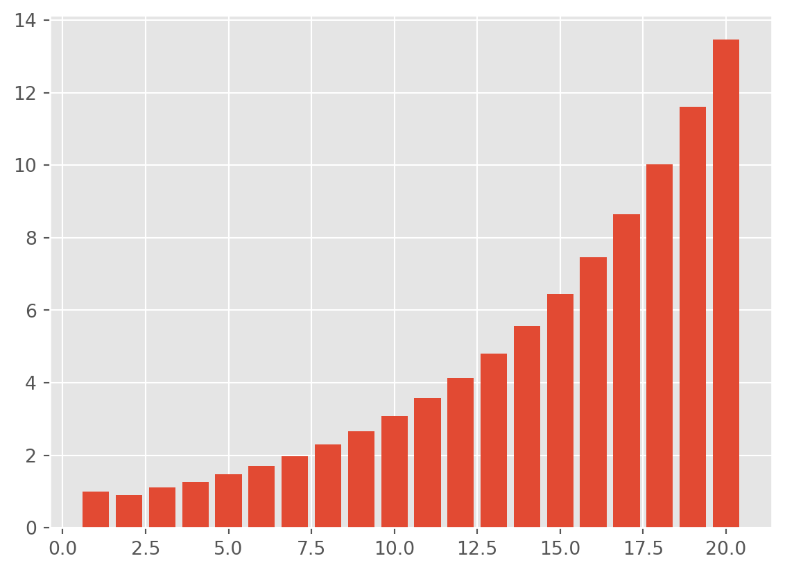
This is an explosive system, since one of eigenvalue is larger than \(1\). However let’s take a look at the graph below, demonstrating different eigenvalues and corresponding behaviors of the system.They are plotted as functions of \(i\): \(f(i)= c_1 \lambda_1^{i-1}+c_2 \lambda_2^{i-1}\)
i = np.arange(1, 50)

lamda1 = [0.99, 1.1, -0.9, -1.2]
lamda2 = [0.01, -1.1, 1.1, 0.4]
c1 = 0.99
c2 = 1 - c1

fig = plt.figure(figsize=(12, 7))
ax_pos = [221, 222, 223, 224]

for j in range(4):
    ax = fig.add_subplot(ax_pos[j])
    pypu1 = c1 * lamda1[j] ** (i - 1) + c2 * lamda2[j] ** (i - 1)
    ax.bar(np.arange(len(pypu1)) + 1, pypu1)
    tt = "$\lambda_1 = %.3f,\ \lambda_2 = %.3f$" % (lamda1[j], lamda2[j])
    ax.set_title(tt, size=13, color="r")
plt.suptitle(
    "$\partial y_{t+i}/\partial u_t = c_1 \lambda_1^{i-1}+c_2 \lambda_2^{i-1}, c_1 = %.3f, c_2 = %.3f$"
    % (c1, c2),
    size=20,
    color="b",
    x=0.5,
    y=1.005,
)
plt.show()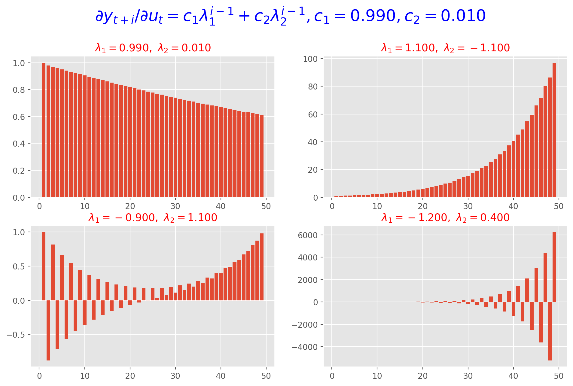
The Dynamic Multiplier of \(3rd\)-Order Difference Equation
Suppose the dynamic multiplier is \(f(i)= c_1 \lambda_1^{i-1}+c_2 \lambda_2^{i-1}+c_3 \lambda_3^{i-1}\)
i = np.arange(1, 50)

lambda1 = [0.6, 1.1, -0.2, -1.2]
lambda2 = [0.01, -1.1, 1.3, -0.4]
lambda3 = [1.01, 0.1, -1.1, 0.9]

c1 = 0.23
c2 = 0.58
c3 = 1 - c1 - c2

fig = plt.figure(figsize=(12, 7))
ax_pos = [221, 222, 223, 224]

for j in range(4):
    ax = fig.add_subplot(ax_pos[j])
    pypu1 = (
        c1 * lambda1[j] ** (i - 1)
        + c2 * lambda2[j] ** (i - 1)
        + c3 * lambda3[j] ** (i - 1)
    )
    ax.bar(np.arange(len(pypu1)) + 1, pypu1)
    tt = "$\lambda_1 = %.3f,\ \lambda_2 = %.3f,\ \lambda_3 = %.3f$" % (
        lambda1[j],
        lambda2[j],
        lambda3[j],
    )
    ax.set_title(tt, size=13, color="r")
plt.suptitle(
    "$\partial y_{t+i}/\partial u_t = c_1 \lambda_1^{i-1}+c_2 \lambda_2^{i-1}+c_3 \lambda_3^{i-1}, c_1 = %.3f, c_2 = %.3f, c_3 = %.3f$"
    % (c1, c2, c3),
    size=22,
    color="b",
    x=0.5,
    y=1.005,
)
plt.show()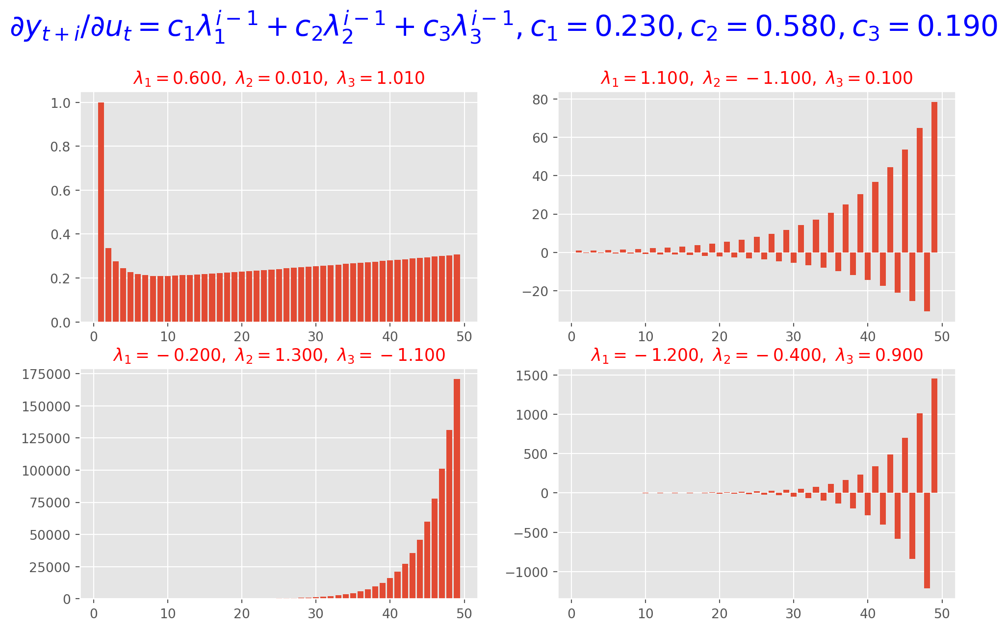
In summary, as long as one of eigenvalues \(|\lambda_i|>1\), dynamic multiplier will eventually be explosive which in turn causing \(y_t\) explosive.
Impulse Response Function of AR(k)
Here we reproduce the example from above \[ Y_t = 0.94 Y_{t-1} - 0.35 Y_{t-2} -0.3 Y_{t-3} +u_t \] The matrix form is \[ \left[\begin{array}{c} Y_t \\ Y_{t-1} \\ Y_{t-2} \end{array}\right]=\left[\begin{array}{ccc} 0.94 & -0.35 & -0.3 \\ 1 & 0 & 0 \\ 0 & 1 & 0 \end{array}\right]\left[\begin{array}{l} Y_{t-1} \\ Y_{t-2} \\ Y_{t-3} \end{array}\right]+\left[\begin{array}{c} u_t \\ 0 \\ 0 \end{array}\right] \]
In short form \[ Z_t = \Lambda Z_{t-1} + \varepsilon_t \]
Except \(\Lambda^0\) defined as an identity matrix \[ \Lambda^0=\left[\begin{array}{lll} 1 & 0 & 0 \\ 0 & 1 & 0 \\ 0 & 0 & 1 \end{array}\right] \]
All \(\Lambda^k\)’s are defined as \[ \left[\begin{array}{ccc} 0.94 & -0.35 & -0.3\\ 1 & 0 & 0 \\ 0 & 1 & 0 \end{array}\right]^j \] And the \((1, 1)\) element is the IRF at the horizon \(j\).
Lambda = np.array([[0.94, -0.35, -0.3], [1, 0, 0], [0, 1, 0]])
irf = []
for i in range(50):
    Lambdai = np.linalg.matrix_power(Lambda, i)
    irf.append(Lambdai[0, 0])

fig, ax = plt.subplots(figsize=(12, 6))
ax.plot(np.arange(len(irf)), irf)
ax.bar(np.arange(len(irf)), irf, color="Coral")
ax.set_title(r"IRF of $Y_t = 0.94 Y_{t-1} - 0.35 Y_{t-2} -0.3 Y_{t-3} +u_t$")
plt.show()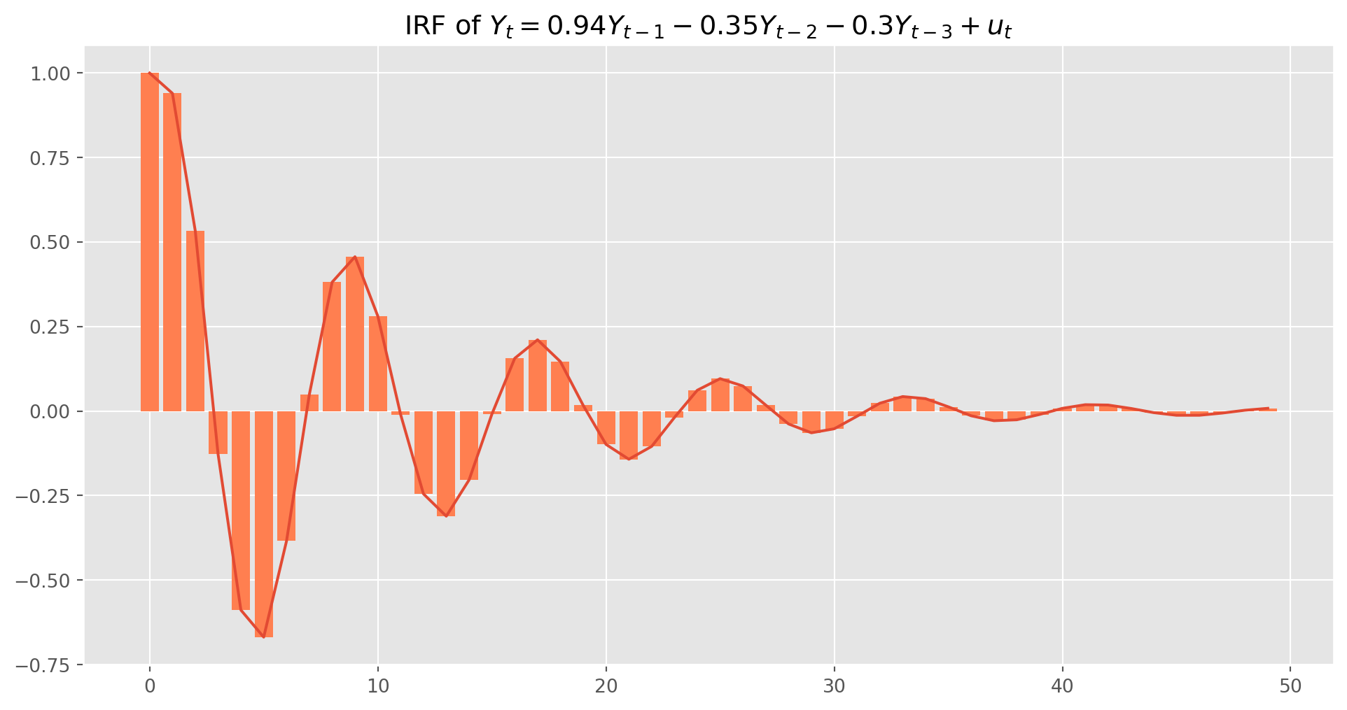
Complex Eigenvalues and Business Cycle Measuring
We are solving the eigenvalues of \(2nd\) order difference equation, we resort to the formulae
\[ \lambda_1=\frac{\phi_1+\sqrt{\phi_1^2+4\phi_2}}{2}\\ \lambda_2=\frac{\phi_1-\sqrt{\phi_1^2+4\phi_2}}{2} \]
However, there is a case of complex solution, i.e. \[ \phi_1^2 + 4\phi_2 <0 \] The eigenvalues are complex conjugates written as \[ \lambda_1=a+bi\\ \lambda_2=a-bi \] where \(i=\sqrt{-1}\).
As a complex solution example, let’s set \(\phi_1=1.5\) and \(\phi_2=-0.8\), use the formula to confirm there is complex solution
1.5**2 + 4 * (-0.8)-0.9500000000000002If the eigenvalues are complex conjugates, the plot of ACF or \(y_t\) will either show the a picture of wavy damping or exploding, hinges on if the modulus of the conjugates less then unit or not, i.e. \(\sqrt{a^2+b^2}<1\).
We will not dive in mathematics of complex numbers, but here is a simulated \(\text{AR(2)}\) plot with the assumed parameters, \(\phi_1=1.5\) and \(\phi_2=-0.8\)
ar_params = np.array([1, -1.5, 0.8])  # alwasy specify zero lag as 1
ma_params = np.array([1])  # alwasy specify zero lag as 1
ar1 = ArmaProcess(ar_params, ma_params)  # the Class requires AR and MA's parameters
ar1_sim = ar1.generate_sample(nsample=100)
ar1_sim = pd.DataFrame(ar1_sim, columns=["AR(1)"])
ar1_acf = acf_func(ar1_sim.values, fft=False, nlags=100)  # return the numerical ACF
fig, ax = plt.subplots(figsize=(12, 5))
ax.bar(np.arange(len(ar1_acf)), ar1_acf, color="tomato", label="AR(1) autocorrelation")
plt.show()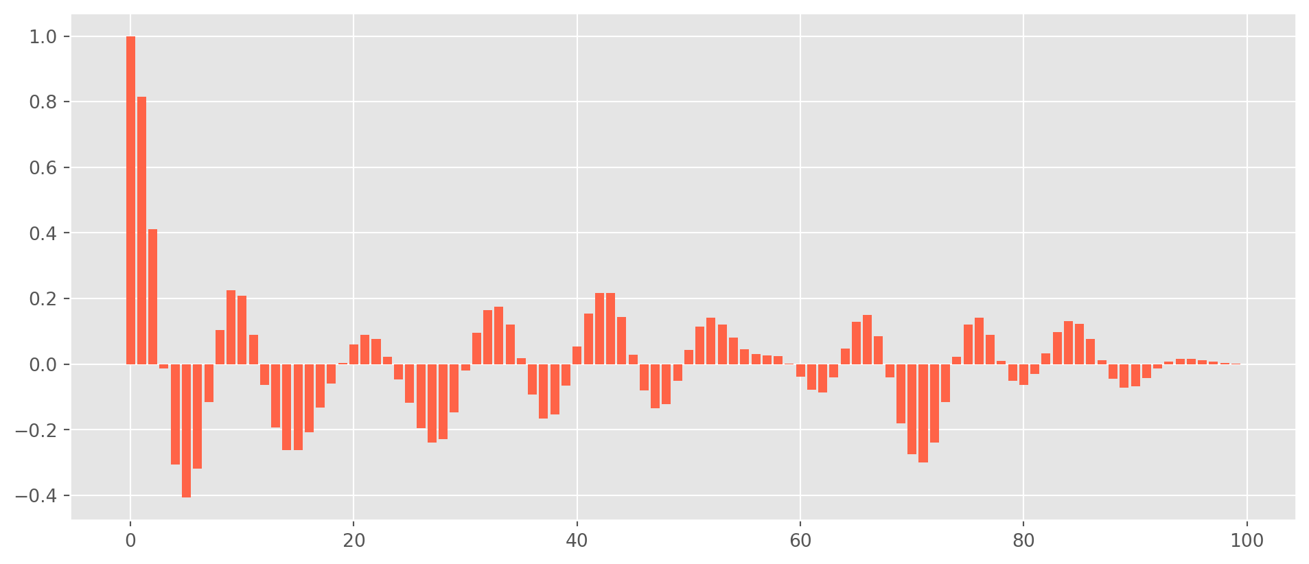
In practice, the complex conjugates characterize the behavior of business cycles to some extent, though not a popular method.
start = dt.datetime(1950, 1, 1)
end = dt.datetime(1995, 2, 1)
# real GDP per cap, gross investment, export, personal consumtpion expenditure
df = data.DataReader(["GDP"], "fred", start, end)
df.columns = ["GDP"]
df_log_diff = (np.log(df) - np.log(df.shift())).dropna()
df_log_diff.plot()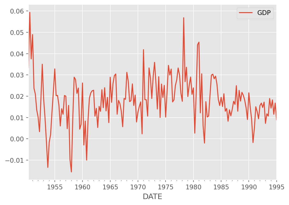
g1 = plot_acf(df_log_diff, zero=False)
g2 = plot_pacf(df_log_diff, zero=False)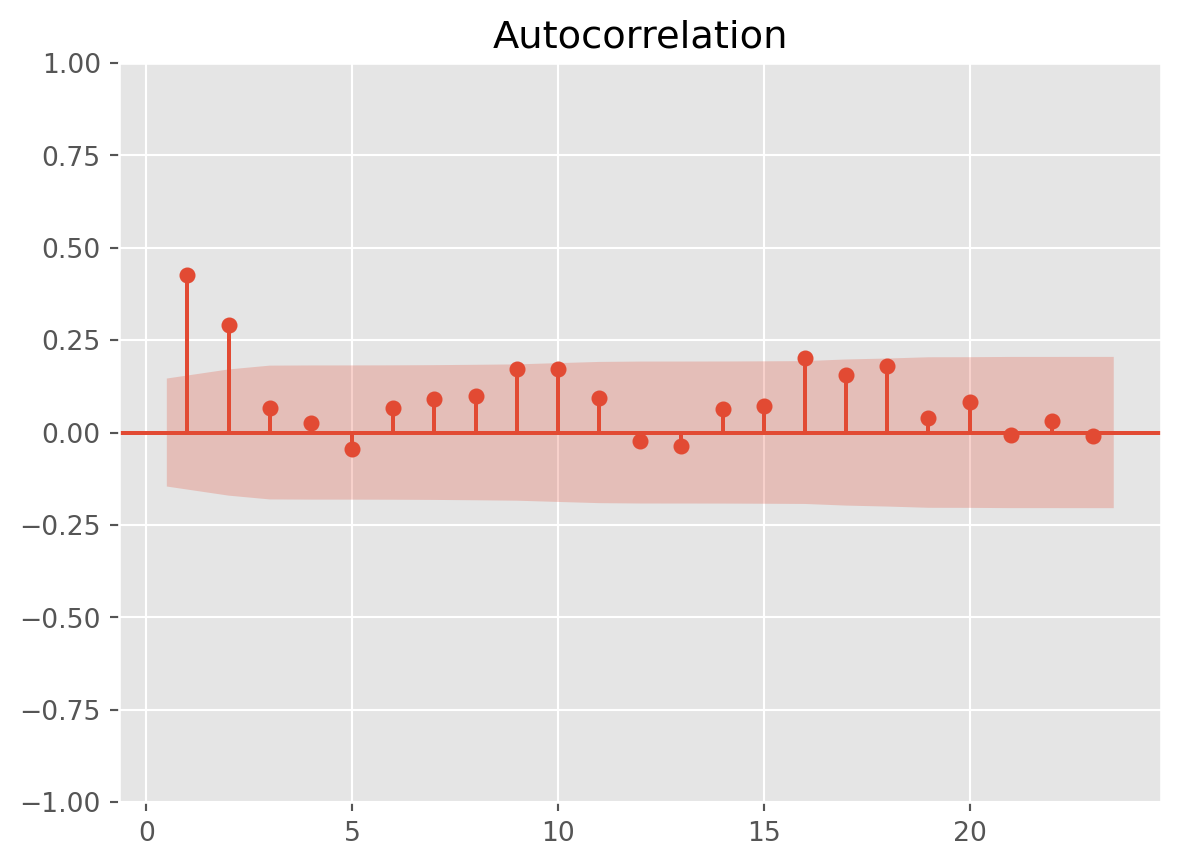
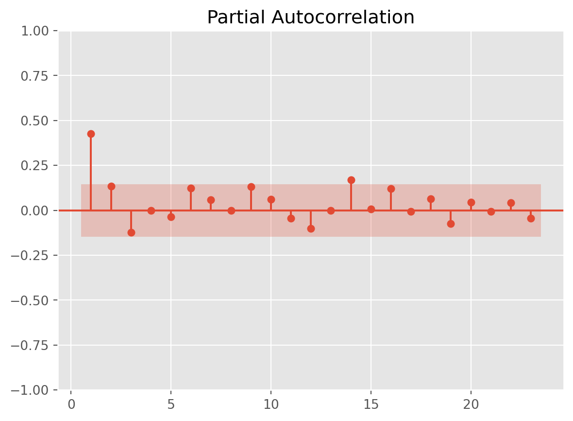
mod_obj = ARIMA(df_log_diff, order=(2, 0, 0))
results = mod_obj.fit()
print(results.summary())
SARIMAX Results
==============================================================================
Dep. Variable: GDP No. Observations: 180
Model: ARIMA(2, 0, 0) Log Likelihood 574.260
Date: Sun, 27 Oct 2024 AIC -1140.521
Time: 17:39:28 BIC -1127.749
Sample: 04-01-1950 HQIC -1135.342
- 01-01-1995
Covariance Type: opg
==============================================================================
coef std err z P>|z| [0.025 0.975]
------------------------------------------------------------------------------
const 0.0184 0.002 11.639 0.000 0.015 0.021
ar.L1 0.3625 0.068 5.319 0.000 0.229 0.496
ar.L2 0.1630 0.066 2.451 0.014 0.033 0.293
sigma2 9.895e-05 8.13e-06 12.168 0.000 8.3e-05 0.000
===================================================================================
Ljung-Box (L1) (Q): 0.11 Jarque-Bera (JB): 27.35
Prob(Q): 0.74 Prob(JB): 0.00
Heteroskedasticity (H): 0.51 Skew: 0.47
Prob(H) (two-sided): 0.01 Kurtosis: 4.66
===================================================================================
Warnings:
[1] Covariance matrix calculated using the outer product of gradients (complex-step).\[ y_t = 0.0155 + 0.4134 y_{t-1} + 0.2012 y_{t-2} + u_t \]